Machine learning is a field of study in the broad spectrum of artificial intelligence (AI) that can make predictions using data without being explicitly programmed to do so. Machine learning algorithms are used in a wide variety of applications, such as recommendation engines, computer vision, spam filtering and so much more. They perform extraordinary well where it is difficult or infeasible to develop conventional algorithms to perform the needed tasks.

机器学习是广泛的人工智能(AI)研究领域，可以使用数据进行预测，而无需进行明确的编程。 机器学习算法被广泛用于各种应用程序中，例如推荐引擎，计算机视觉，垃圾邮件过滤等等。 在难以或无法开发常规算法来执行所需任务的情况下，它们的性能非常出色。

While many machine learning algorithms have been around for a long time, the ability to automatically apply complex mathematical calculations to big data— over and over, faster and faster — is a recent development.

尽管许多机器学习算法已经存在很长时间了，但是自动将复杂的数学计算自动应用于大数据的能力(一遍又一遍，越来越快)是最近的发展。

One of the most overwhelmingly represented machine learning techniques is a neural network. Since intelligence is foremost human, insights from the human mind were derived in order to create intelligent machines. It is based on the idea of a neuron. I assume you’re already familiar with the basics of how neural networks work and won’t go into much detail on the architecture.

神经网络是压倒性代表最多的机器学习技术之一。 由于智能是人类的头等大事，因此从人类思想中得出的见解就是为了创造智能机器。 它基于神经元的思想。 我假设您已经熟悉了神经网络的工作原理，并且不会在体系结构上做太多详细介绍。

Once the model trains, a metrics has to be defined to measure the model performance i.e the loss or cost function. There is not a single uniform loss function that we could apply in each case. Each serves its own purpose. For example, we could be using a cats versus dogs data and would therefore need a binary loss that outputs the possibility of it being a dog or a cat. And so long for tasks, such as multiclass classification, linear regression, clustering algorithms etc. In some cases, a custom loss function is required.

一旦训练了模型，就必须定义一个度量来测量模型性能，即损失或成本函数。 在每种情况下都没有一个统一的损失函数可以应用。 每个都有自己的目的。 例如，我们可能使用的是猫与狗的数据，因此需要二进制损失来输出它可能是狗还是猫的可能性。 并且对于诸如多类分类，线性回归，聚类算法等任务的时间如此长。在某些情况下，需要自定义损失函数。

The optimizer’s job is to optimize the weights and biases so that the loss is minimized. How could we achieve this?

优化器的工作是优化权重和偏差，以使损失最小化。 我们如何实现这一目标？

Let me introduce you to gradient descent!

让我向您介绍梯度下降！

Given a loss function [J] we can calculate the partial derivatives of J by the weight matrix. Note: gradient vector of the function shows in the direction of steepest ascent. Check https://www.khanacademy.org/math/multivariable-calculus or any other source.

给定损失函数[J]，我们可以通过权重矩阵计算J的偏导数。 注意：函数的梯度向量以最陡峭的上升方向显示。 检查https://www.khanacademy.org/math/multivariable-calculus或任何其他来源。

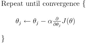
Since our goal is to find the point where loss is minimised (this point is also reffered to as the global minimum) all we have to do is to go in the exact opposite direction.

因为我们的目标是找到使损失最小化的点(该点也称为全局最小值)，所以我们要做的就是朝着完全相反的方向前进。

Here, we introduce a hyperparameter called the learning rate, which determines the step size at each iteration and should be set between 0 and 1. It ultimately represents the speed at which the model learns.

在这里，我们引入了一个称为学习率的超参数，该参数确定每次迭代的步长，并且应将其设置为0到1。它最终代表了模型学习的速度。

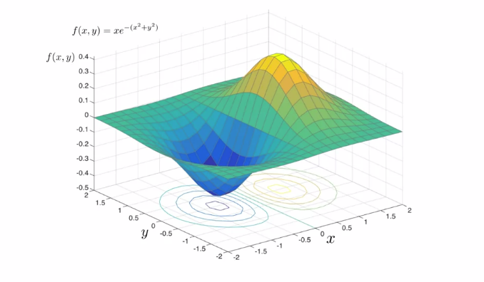
Pretty straightforward, right? Except for one thing. The loss function is never as simple as shown above. In reality, it’s closer to this:

很简单吧？ 除了一件事。 损失函数从来没有像上面所示的那么简单。 实际上，它更接近于此：

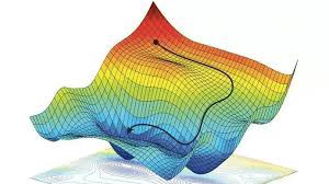
It has many local minima in which the optimizer might get stuck in.

它具有许多局部最小值，优化器可能会陷入其中。

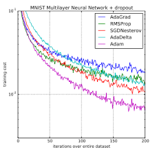
Training a very large dense neural network can be painfully slow. Huge speed boost comes from using a faster optimizer than the plain ‘vanilla’ gradient descent. We will unveil some of the best performing optimization algorithms out there.

训练非常大的密集神经网络可能会非常缓慢。 与普通的“香草”梯度下降相比，使用更快的优化器可以极大地提高速度。 我们将推出一些性能最佳的优化算法。

Recall that gradient descent simply updates the weights by subtracting the gradient of the cost function J(θ) with regards to the weights matrix multiplied by the learning rate η. The equation is: θ ← θ — η? θ J(θ). It does not care about what the earlier gradients were. If the local gradient is tiny, it goes very slowly.

回想一下，梯度下降只是通过将权重矩阵乘以学习率η减去成本函数J(θ)的梯度来简单地更新权重。 公式为：θ←θ—η?θJ(θ)。 它不在乎早期的渐变是什么。 如果局部渐变很小，则渐变会非常缓慢。

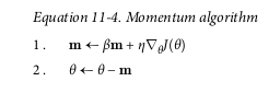
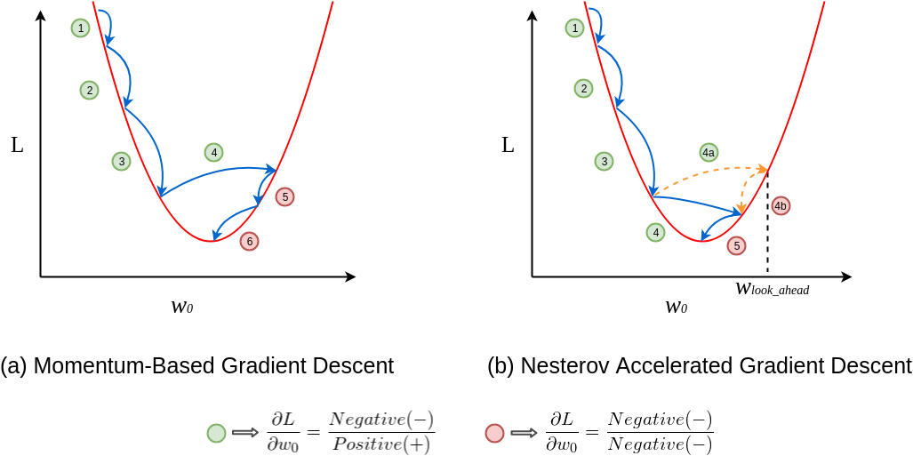
Momentum optimization solves this by adding the local gradient*learning rate to the momentum vector m. It helps accelerate gradients vectors in the right directions, thus leading to faster converging. This allows Momentum optimization to escape from plateau much faster than Gradient Descent. It can also help roll past local minima.

动量优化通过将局部梯度*学习率添加到动量矢量m来解决此问题。 它有助于在正确的方向上加速梯度矢量，从而加快收敛速度。 这使得动量优化比梯度下降要快得多地从高原逃逸。 它还可以帮助解决本地最低要求。

To prevent the momentum from growing too large, the algorithm introduces a new hyperparameter β, which must be set between 0 and 1. A typical momentum value is 0.9.

为了防止动量过大，该算法引入了一个新的超参数β，该超参数必须设置为0到1。典型的动量值为0.9。

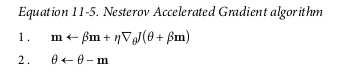
The idea of Nesterov Momentum optimization, or Nesterov Accelerated Gradient (NAG), is to measure the gradient of the cost function not at the local position but slightly ahead in the direction of the momentum. The only difference from vanilla Momentum optimization is that the gradient is measured at θ + βm rather than at θ.

Nesterov动量优化或Nesterov加速梯度(NAG)的想法是测量成本函数的梯度，而不是在局部位置，而是在动量方向上稍稍领先。 与香草动量优化的唯一区别是，梯度是在θ+βm而不是θ处测量的。

The nesterov update ends up slightly closer to the optimum.

Nesterov更新最终会稍微接近最佳结果。

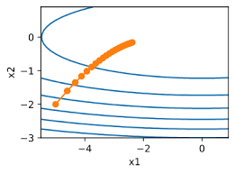
Imagine this scenario again. A ball going down the elongated bowl. No real loss function will be this neatly constructed but for the sake of explanation, follow along. Gradient descent starts by quickly going down the steepest slope, then slowly goes down the bottom of the valley. It would be nice if the algorithm could detect this early and correct its direction to point a bit more toward a global minimum.

想像再次出现这种情况。 球从细长的碗中掉下来。 不会如此巧妙地构建任何实际的损失函数，但是为了解释起见，请遵循。 梯度下降首先从最陡峭的斜坡下降，然后缓慢地下降到谷底。 如果该算法可以及早发现并纠正其方向，使其指向全局最小值，那将是很好的。

The AdaGrad algorithm achieves this by scaling down the gradient vector along the steepest dimension.

AdaGrad算法通过沿最陡峭的维度按比例缩小梯度矢量来实现此目的。

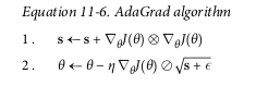
Vector s stores the square of the gradients. In other words, the vector s accumulates the squares of the partial derivatives of the cost function. If the cost function is steep along the i-th dimension, then s will get larger and larger at each iteration.

向量s存储渐变的平方。 换句话说，向量s累积成本函数偏导数的平方。 如果成本函数沿第i个维度陡峭，则s将在每次迭代中变得越来越大。

The second step is identical to gradient descent. The gradient vector is scaled down by a factor of the root of s +ε where ε is a smoothing term to avoid division by zero, typically set to 10 –10 .

第二步与梯度下降相同。 梯度矢量按s +ε的根比例缩小，其中ε是避免除以零的平滑项，通常设置为10 –10。

In short, this algorithm decays the learning rate, but it does so faster for steep dimensions than for dimensions with gentler slopes. This is called an adaptive learning rate. It helps point the resulting updates more directly toward the global optimum. One additional benefit is that it requires much less tuning of the learning rate hyperparameter η.

简而言之，该算法会降低学习速度，但是对于陡峭的尺寸，它的速度要比斜率较小的尺寸的学习速度快。 这称为自适应学习率。 它有助于将结果更新更直接地指向全局最优值。 另一个好处是，它需要学习速率超参数η的调整要少得多。

Often the learning rate gets scaled down so much that the algorithm ends up stopping entirely before reaching the global minimum.

通常，学习率会被缩小得如此之大，以至于算法最终在达到全局最小值之前就完全停止了。

RMSProp fixes this by accumulating only the gradients from the most recent iterations(as opposed to all since the training began).

RMSProp通过仅累积最近一次迭代中的梯度(而不是自训练开始以来的所有梯度)来解决此问题。

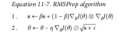
The decay rate β is typically set to 0.9. Yes, it is once again a new hyperparameter, but this default value often works well, so you may not need to tune it at all.

衰减率β通常设置为0.9。 是的，它再次是一个新的超参数，但是此默认值通常效果很好，因此您可能根本不需要调整它。

Adam stands for Adaptive Moment estimation and combines the idea of momentum optimization (i.e holding the values of gradients in a vector) and RMSProp (keeping track of an exponentially decaying average of past squared gradients).

亚当(Adam)代表自适应矩估计，它结合了动量优化(即，将梯度的值保存在矢量中)和RMSProp(跟踪过去平方梯度的指数衰减平均值)的思想。

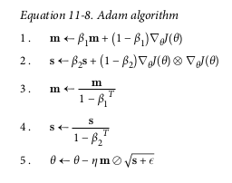
Since Adam is an adaptive learning rate algorithm much like AdaGrad and RMSprop it requires less tuning of the learning rate.

由于Adam是一种自适应学习速率算法，非常类似于AdaGrad和RMSprop，因此它需要较少的学习速率调整。

In this jupyter notebook I am using the CIFAR-10 image classification dataset with Tensorflow. I’m sampling down to size 10000. Don’t mind how the model is instantiated, but the hyperparameters are the same for each time the model uses different optimizers. We pass the optimizer along with the metrics and loss measuring performance to the model.compile method.

在此Jupyter笔记本中，我将使用带有Tensorflow的CIFAR-10图像分类数据集。 我采样到的大小为10000。不介意如何实例化模型，但是每次模型使用不同的优化器时，超参数都是相同的。 我们将优化器以及指标和损耗测量性能传递给model.compile方法。

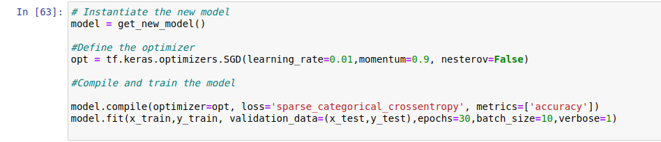
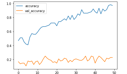
Here, I’ve used the Momentum optimization with the momentum of 0.9 and it achieved an accuracy of 91%. Note that setting the Nesterov Accelerated Gradient is as simple as setting the boolean nesterov to true. As stated before the Nesterov almost always outperforms Momentum optimization. It reached an accuracy of 93%. Since I am using a relatively small dataset, I might have problems overfitting the data.

在这里，我使用动量优化为0.9的动量优化，其精度达到了91％。 请注意，设置Nesterov Accelerated Gradient就像将布尔Nesterov设置为true一样简单。 如前所述，内斯特罗夫几乎总是胜过动量优化。 准确度达到93％。 由于我使用的是相对较小的数据集，因此我可能会在数据过度拟合方面遇到问题。

Next is the Adagrad optimizer. Again, tensorflow makes it super easy to implement it with the high-level keras API.

接下来是Adagrad优化器。 同样，tensorflow使使用高级keras API轻松实现它。

The epsilon is the parameter that prevents dividing with zero. I’ve used the default value. Adagrad reached an accuracy of 82.1%.

epsilon是防止除以零的参数。 我使用了默认值。 Adagrad的准确度达到82.1％。

RMSprop is yet another no-brainer.

RMSprop是另一个明智的选择。

Note the rho parameter which is the decay rate. Its default value is 0.9. RMSprop didn’t dissapoint and reached an accuracy of 96.4%.

注意rho参数，它是衰减率。 其默认值为0.9。 RMSprop并未感到失望，并且达到了96.4％的准确性。

And finally, the Adam optimizer. You can check the parameters passed to the Adam optimizer on the Tensorflow website (https://www.tensorflow.org/api_docs/python/tf/keras/optimizers/Adam), but I’ll leave the defaults.

最后是Adam优化器。 您可以在Tensorflow网站( https://www.tensorflow.org/api_docs/python/tf/keras/optimizers/Adam )上检查传递给Adam优化器的参数，但我将保留默认值。

Instead of initializing optimizers this way, you can write this:

不用这样初始化优化器，您可以这样编写：

Tensorflow will reffer to the default values of the adam optimizer.

Tensorflow将恢复为adam优化器的默认值。

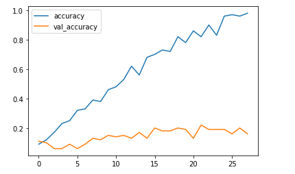
The Adam optimizer reached training accuracy of 98.0%.

Adam优化器的训练精度达到98.0％。

In conclusion, optimization algorithms have a crucial role in the process of model training and performance. I have lead you through the idea of plain gradient descent, which takes the partial derivatives of the cost function to determine what the right step to reach the local mininum is and continued with storing past gradients in a vector, so that the convergence takes place faster. Then with AdaGrad scaling down the gradient vector along the steepest dimension and introduced you to adaptive learning rate to finally arrive at the ultimate optimization algorithm, which combines both the exponentially decaying average and the past gradients.

总之，优化算法在模型训练和性能过程中具有至关重要的作用。 我已经引导您完成了纯梯度下降的想法，该想法采用成本函数的偏导数来确定达到局部最小值的正确步骤，并继续将过去的梯度存储在向量中，以便更快地进行收敛。 。 然后，使用AdaGrad沿最陡峭的维度按比例缩小梯度矢量，并向您介绍自适应学习率，最终得出最终的优化算法，该算法将指数衰减的平均值和过去的梯度结合在一起。

Citation: Ge?ron, A. (2017). Hands-on machine learning with Scikit-Learn and TensorFlow : concepts, tools, and techniques to build intelligent systems. Sebastopol, CA: O’Reilly Media. ISBN: 978–1491962299

引文：盖伦·A(2017)。 使用Scikit-Learn和TensorFlow进行动手机器学习：构建智能系统的概念，工具和技术。 加利福尼亚塞巴斯托波尔：O'Reilly Media。 国际标准书号(ISBN)：978–1491962299